Probabilistic Models of Film Reciprocity Failure
Introduction
This article is the next iteration in my saga of diving down the film photography rabbit hole. We’ll begin by discussing the topic of exposure from the perspective of a photographer before diving into the physics and mathematics underlying their experience.
Film Exposure - The Law of Reciprocity
When shooting on film, it is important that the film is properly exposed - meaning it receives the proper amount of light. Images which are overexposed appear bright and washed out, whereas underexposed images are dark and undefined.
From a photograph’s perspective, properly exposing an image is a function with three parameters - film speed (ISO), aperture, and shutter speed. In short, film speed is a fixed value depending on the film stock used (e.g. Portra 400, Provia 100, etc) where higher numbers indicated higher sensitivity to light. Aperture determines the amount of light which enters the camera during exposure, and shutter speed determines how long the film is exposed for. Under normal circumstances, the amount which an image is “exposed” is the product of aperture and shutter speed. For example, cutting the aperture in half (e.g. from 2.8 to 5.6) requires exposing the image for twice as long to get the same exposure. The conditions under which exposure is determined as the product of aperture and time is referred to as the law of reciprocity.
Photographers shooting handheld will often experience this during low-light conditions. When shooting without a tripod, most SLR cameras with a shutter speed of less than 1/60th of a second will shake enough to create a blurry image. If your light meter reads that you should use an aperture of 3.6 at 1/30th of a second, you can open your aperture to 1.8 (doubling it’s size) and use a shutter speed of 1/60th of a second to generate the same exposure.
Reciprocity Failure
Under most shooting conditions, the law of reciprocity mentioned above holds true. During periods of exceptionally high or low light, however, the law or reciprocity breaks down - this is known as reciprocity failure. Most photographers will experience this during extremely low-light photography, such as astrophotography. When shooting at night, film must be exposed for increasingly longer periods of time, implying that the total exposure is not a product of light intensity and exposure time when the intensity is exceptionally low.
As an example, suppose you are shooting Ilford HP5+, which has a box-speed rating of 400 ISO. Taking a reading with a light meter, which assumes that the law of reciprocity holds, indicates that you should expose for 10 seconds. Using a table provided by Ilford to account for reciprocity failure, however, indicates that this value should be corrected to 20.4 seconds to account for the decreased efficiency of the film at such low light intensities.
This article will attempt to understand what causes low-intensity reciprocity failure and explain the mathematics behind it.
Note: reciprocity failure appears both during exceptionally high intensity conditions and low intensity conditions. The former, however, is only applicable in certain scientific scenarios such as lasers and hence will not be the subject of this article.
The Gurney-Mott Hypothesis
Before we dive into the mathematics of calculating reciprocity failure curves, we need to understand how film captures light and what underlying mechanism is responsible for reciprocity failure.
At a very high level, The Gruney-Mott hypothesis describes film as being made of silver ions in a gelatin or plastic medium which are arranged in grains. These silver ions interact with photons in order to form silver atoms - those with a net neutral charge - which are stable and can be developed. Interestingly, a silver ion must interact with two photons in order to become a silver atom. Once a photon has struck a silver ion it enters an intermediate state where it will decay after some time. If the second photon arrives within this time interval a stable silver atom is formed, otherwise the atom decays back into the ionic state and must be hit with two photos again within the time interval in order to be developed.
For a more technical description of the Gruney-Mott Hypothesis, read this dropdown...
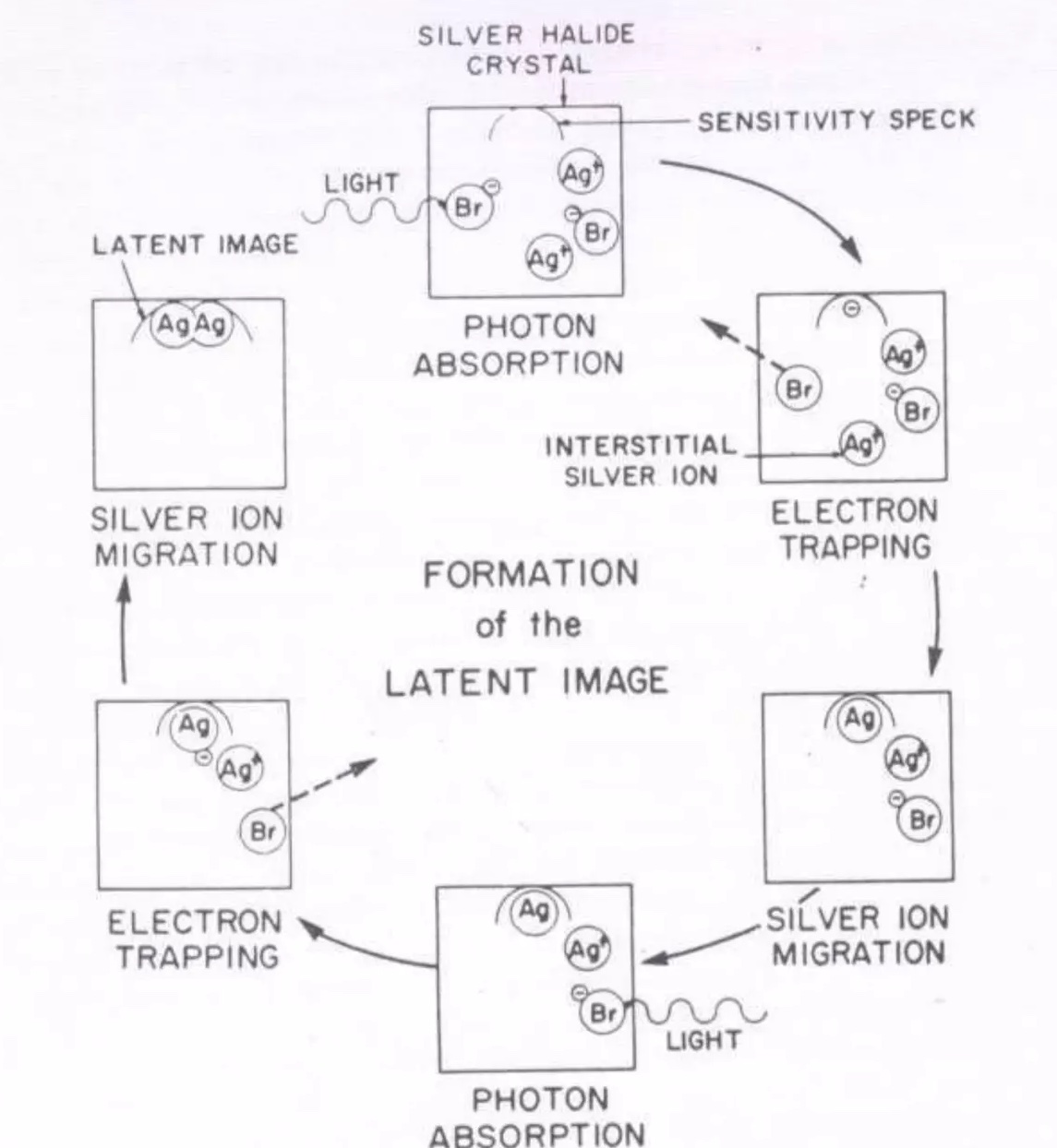
Film is made of a thin photographic emulsion coated on a support medium such as plastic. The emulsion itself is made of small grains, which contains a number of free-floating ions (recall from chemistry that an ion is an atom with a net electrical charge). Most photographic film uses silver ions, \(Ag^+\), and optionally some sort of halide (a negatively charged Halogen) such as Bromide. Finally, each grain contains a sensitivity spec where the latent image will be formed.
When the emulsion is exposed to light, photons interact with the ions in the grain to generate electron hole pairs which float independently throughout the grain. These are called photoelectrons.
When a photoelectron finds the sensitivity spec it will become stuck, generating a potential field around it which attracts interstitial silver ions.
When an interstitial silver ion arrives at the spec it becomes a silver atom with no net charge. Importantly, the silver atom at the sensitivity spec is only stable for a short period of time. After some time, which we will denote as \(r_0\), the atom decays back into an electron and a silver ion.
However, if the silver atom from the previous step is joined by another silver atom before it has time to decay, the sensitivity spec will be stable and becomes a latent image - something that can be developed into a permanent, non-light-sensitive picture.
The decay time, \(r_0\) is ultimately the mechanism which is responsible for low-intensity reciprocity failure. Once the exposure time exceeds \(r_0\) the photographic process becomes less efficient as some grains will decay before they have the opportunity to trap the necessary number of silver atoms.
We note that there is some debate as to the critical number of silver atoms which must meet at a sensitivity spec in order to form a stable latent image. For the purpose of this article we will assume that this number is two, which is supported by early research at Kodak Laboratories into film reciprocity failure.
 Could not find the original source for this
Thinking somewhat mathematically, you might imagine that a latent image is formed for a sensitivity spec if, and only if, the spec contains two silver atoms during an interval \(r_0\).
A sprint through probability theory
We will need a baseline understanding of probability theory in order to analyze the Gurney-Mott hypothesis described above.
Discrete Random Variables
Random variables are one of the most poorly named parts of probability theory, as they are neither variables nor are they random. Instead, a random variable is a function (what the fuck) from a sample space to a measurable space. Technically speaking, a sample space is defined by the triplet \((\Omega, F, P)\) and a measurable space is a set and a \(\sigma -algebra\). I don’t believe those concepts really helps us understand random variables, however, so we’ll skip them for now.
Let’s make random variables more concrete by considering an example. Suppose that you conducted an experiment where you flipped a coin three times. Each time you flip heads you win a dollar, and each time you flip heads you lose a dollar. In this case, the sample space is clearly all possible outcomes of the experiment. In other words, \(\Omega = \{\{HHH\}, \{HHT\}, \{HTH\}, \{THH\}, \{HTT\}, \{THT\}, \{TTH\}, \{TTT\} \}\). Then let us define \(X\) as the random variable which represents our winnings. Then, one might say that \(X(HHH) = \$3\).
Note that random variables can be either discrete or continuous, depending on if the image of a random variable \(X\) is countable or not. For the purpose of this article we will only consider discrete random variables going forward.
Probability Mass Function
The probability mass function, pmf, or discrete probability density function, is a function which describes how likely a given random variable is to take on a given value.
I find it easiest to reason about a probability mass function if you consider the space on which it operates. A random variable, \(X\), is a function \(X: \Omega \to E\). A probability mass function, which we might call \(f_X\), is a function \(f_X: E\to [0, 1]\). The key observation to make here is that the \(E\) from the codomain of the random variable \(X\) is the same \(E\) that appears as the domain to the probability mass function \(f_X\).
Again, let’s try to make this concrete by continuing with our previous example. Suppose that our coin was far - meaning that heads is as likely to come up as tails. Then \(f_X (-3) = 1/8 = 0.125 = f_X(3)\). Likewise \(f_X(-1) = 3/8 = 0.375 = f_X(1)\).
Cumulative Distribution Function
A cumulative distribution function, or cdf, is similar to a probability mass function in that operates over the same space - the codomain of some random variable \(X\). Unlike the probability mass function, which computes the probability that \(X\) takes on exactly some value \(k\), the cumulative distribution function computes the probability that \(X\) will take on a value less than or equal to \(k\).
In the case of a discrete random variable, which is what we are interested in for the purpose of this article, the cumulative distribution function is quite easy to define. Let \(F_X(k)\) be the cumulative distribution function over a discrete random variable \(X\), then
\[F_x(k) = P(X \le k) = \sum_{k_i \le k} P(X = k_i)\]A natural corollary of the cumulative distribution function is the complementary cumulative distribution function, or ccdf. Simply put, the ccdf answers the question “how often is a random variable \(X\) above a certain value”. Let \(\bar{F}_{X}\) be the ccdf for a discrete random variable \(X\), then
\[\bar{F}_{X}(k) = P(X > k) = 1 - F_X(k) = 1 - P(X \le k)\]Bernoulli Random Variables
A Bernoulli trial is a random experiment which has exactly two possible outcomes - success or failure. By convention, we usually denote the probability mass function of a Bernoulli random variable with \(1\) as the value indicating a success and \(0\) indicating a failure.
In other words, A random variable has probability of \(p\) for a successful outcome, then the pmf
for \(X\) is given by
The Binomial Distribution
After considering a Bernoulli random variable, it is natural to think about what happens when we repeat a given trial multiple times. A random variable which operates over \(n\) identical Bernoulli trials is known as a Binomial random variable, and is parameterized by a probability of success \(p\) for each trial and \(n\) total trials.
Let’s now try to derive the probability mass function for a Binomial random variable \(X\). First, we note that the probability that exactly \(k\) of the \(n\) trials have a successful outcome is given by \(p^k\). It is important to note here that this is only true since the outcome of each event is independent of all other events. In other words, a successful outcome for the first trial does not impact the probability that the second trial is also successful. Likewise, the probability that the other \(n-k\) events have an unsuccessful outcome is given by \({(1-p)}^{n-k}\). It is not sufficient to simply multiply these two values together, however. We must also consider the number of sequences which contain exactly \(k\) successful outcomes (and hence \(n-k\) failures). This is a common combinatorial problem, given by the aptly named Binomial coefficient. You might think of the Binomial coefficient, \(C(k, n)\), as the number of ways to select \(k\) outcomes from \(n\) total trials.
\[C(k, n) = \frac{n!}{k!(n-k)1} 0 \le k \le n\]Thus, we can say that the probability mass function for a Binomial random variable \(X\) is given by
\[P(X = k) = C(k, n) p^k (1-p)^{n-k} = \binom{n}{k} p^k (1-p)^{n-k}\]Deriving The Poisson Distribution
A Binomial random variable is one which operates over a number of countable trials \(n\). For example, we might consider a Binomial random variable which computes the number of heads that arise when a given coin is flipped. What if, however, we wanted to consider a random process which occurs over a given time interval, where the likelihood of success at any given point in time is near zero, but is some reasonable number over the entire interval. For example, we might want to count the number of meteorites that hit Earth in a given year, or the number of photons that hit a sensor on a telescope. This kind of process is described as Poisson, and it is a special case of the Binomial distribution where the number of trials we conduct tends to infinity.
Let’s attempt to derive the Poisson distribution below.
Recall that a Binomial process is given by the following
\[P(\text{Bin} = k) = \frac{n!}{(n-k)!k!} p^k {(1-p)}^{n-k}\]Before we take any limits, however, let’s first consider the value of \(p\). For some usual Binomial random variable, the probability of success is well defined for a single trial. If we are going to take \(n\) as it tends to infinity, however, the probability that the outcome is successful for any given trial is going to be near zero. Thus, let’s start by defining a constant, \(\lambda\), which represents the number of anticipated successful outcomes over \(n\) trials. In other words, let \(\lambda = n p\).
Let us begin by substituting \(\lambda\) above
\[\begin{align} \frac{n!}{(n-k)!k!} p^k {(1-p)}^{n-k} &= \binom{n}{k} {\left(\frac{\lambda}{n}\right)}^{k} {\left(1 - \frac{\lambda}{n}\right)}^{n-k}\\ \end{align}\]Let’s start to make this more manageable to take the limit of by separating our constants (terms which do not include \(n\)) and non-constants (those that do include \(n\))
\[= \frac{\lambda^k}{k!} \frac{n!}{(n-k)!} \frac{1}{n^k} {\left(1 - \frac{\lambda}{n}\right)}^{n-k}\]To simplify the above notation, let’s independently consider a few of the terms and rewrite them. First, consider the second and third terms
\[\begin{align} \frac{n!}{(n-k)!}\frac{1}{n^k} &= \frac{n(n-1)(n-2)\cdots(n-k+1)(n-k)!}{(n-k)!n^k}\\ &= \frac{n(n-1)(n-2)\cdots(n-k+1)}{n^k}\\ &= \frac{n}{n} \frac{n-1}{n} \frac{n-2}{n} \cdots \frac{n-k+1}{n}\\ &= 1 \left(1 - \frac{1}{n}\right)\left(1 - \frac{2}{n}\right) \cdots \left(1 - \frac{k+1}{n}\right) \end{align}\]Let us also rewrite
\[{\left(1 - \frac{\lambda}{n}\right)}^{n-k} ={\left(1 - \frac{\lambda}{n}\right)}^{n}{\left(1 - \frac{\lambda}{n}\right)}^{-k}\]Rewriting our original equation, we are left with
\[\frac{n!}{(n-k)!k!} p^k {(1-p)}^{n-k} = \frac{\lambda^k}{k!} \left(1 - \frac{1}{n}\right)\left(1 - \frac{2}{n}\right) \cdots \left(1 - \frac{k+1}{n}\right) {\left(1 - \frac{\lambda}{n}\right)}^{n}{\left(1 - \frac{\lambda}{n}\right)}^{-k}\]Finally, let’s take the limit of this equation as \(n\) tends to infinity.
\[\lim_{n\to\infty}\frac{n!}{(n-k)!k!} p^k {(1-p)}^{n-k} = \lim_{n\to\infty}\frac{\lambda^k}{k!} \left(1 - \frac{1}{n}\right)\left(1 - \frac{2}{n}\right) \cdots \left(1 - \frac{k+1}{n}\right) {\left(1 - \frac{\lambda}{n}\right)}^{n}{\left(1 - \frac{\lambda}{n}\right)}^{-k}\]Recall from calculus the product law of limits, which states that
\[\lim_{n\to\infty} \left(f(n)\cdot g(n)\right) = \left(\lim_{n\to\infty} f(n)\right)\left(\lim_{n\to\infty}g(n)\right)\]Therefore, we can independently evaluate the limits of the simplifications described above and take their product.
Let us consider the first non-constant terms
\[\lim_{n\to\infty} \left(1 - \frac{1}{n}\right)\left(1 - \frac{2}{n}\right) \cdots \left(1 - \frac{k+1}{n}\right)\]For each term of this sequence, the value of \(\frac{k}{n}\) approaches zero as \(n\) tends to infinity. Thus, the value of each term has a limit of one, implying that
\[\lim_{n\to\infty} \left(1 - \frac{1}{n}\right)\left(1 - \frac{2}{n}\right) \cdots \left(1 - \frac{k+1}{n}\right) = 1\]Then we consider the following terms
\[\lim_{n\to\infty}{\left(1 - \frac{\lambda}{n}\right)}^{n}{\left(1 - \frac{\lambda}{n}\right)}^{-k}\]The leftmost term is defined as \(e^{-\lambda}\). The rightmost term tends to one for the same reason the previous terms did.
Thus, we can rewrite our original limit as following:
\[\lim_{n\to\infty}\frac{n!}{(n-k)!k!} p^k {(1-p)}^{n-k} = \frac{\lambda^k e^{-\lambda}}{k!}\]Thus, a Poisson random variable \(X\) is parameterized by \(\lambda > 0\), with a probability mass function parameterized by \(\lambda >0\) and \(k\) occurrences of the event, defined by
\[P(X = k) = \frac{\lambda^k e^{-\lambda}}{k!}\]Mathematical Modeling
The goal for the rest of this article will be the reconcile, to the best of our ability, the experimental findings of reciprocity failure with a mathematical understanding of the Gurney-Mott hypothesis described above.
Without Reciprocity Failure
Let’s begin by defining a random variable \(R\) which denotes the number of photons absorbed by a grain over some period of time. We can treat photons as discrete units (apologies to any physicists reading this), and we can simply treat the grain, along with it’s Silver Bromide lattice, as described by the Gurney-Mott hypothesis above as a single entity which absorbs photons.
First, the probability that the grain shall absorb exactly \(k\) photons is given by the Possion probability mass function below
\[P(R = k) = \frac{\lambda^{k} e^{-\lambda}}{k!}\]We define \(\lambda\) as a function of the expected number of quanta that a grain is exposed to over the duration of the exposure. We will make the restriction that the intensity and aperture of photo is constant over the exposure time. In the literature, \(\lambda\) is often defined as \(\epsilon a n\), where \(\epsilon\) is the efficiency of the grain in absorbing photons, \(a\) is the area of the grain, and \(n\) is the number of photons released over a time \(t\). As the reader can probably tell, however, \(\epsilon\) and \(a\) are constants, and so it is necessary to say only that \(\lambda\) is some function of \(n\) for now.
Thus, the probability that \(R\) absorbs \(k\) or more photons is given by the following complementary cumulative distribution function
\[P(R \ge k) = 1 - e^{\lambda}\left[1 + \lambda + \frac{1}{2!}\lambda^2 + \cdots + \frac{1}{(k-1)!}\lambda^{k-1}\right]\]Using the theory of the Gurney-Mott hypothesis above, we can take \(k = 2\), meaning that two photons are necessary to create a developable grain, and arrive at the following
\[P(R \ge 2) = 1 - e^{\lambda}(1 + \lambda)\]Now, consider that \(\lambda = cn\), where \(c\) is some constant as mentioned above. Then the probable number of developable grains is a function of \(n\) alone, where \(n\) denotes the number of quanta the grain can be exposed to. If we take \(n = it\), where \(i\) denotes the aperture of the lens (intensity) and \(t\) denotes the time of exposure, then it is clear the law of reciprocity is modeled by the above equation. Halving the value of \(i\) would require doubling the value of \(t\) in order to have the same probability of a developable a grain.
With Reciprocity Failure
Lovely, we now have a simple model which reflects the behavior of the system at moderate intensities. But, as mentioned earlier, let’s attempt to account for reciprocity failure. Defined mathematically, we will say that a grain is developable if, and only if, the grain is struck by two photons within an interval \(\tau\). Otherwise we assume the first photon has decayed and the sensitivity spec in the grain no longer contains a silver atom.
Let’s begin by considering values for \(t_1\), which we will denote as the total time the emulsion is exposed for (the use of a subscript will be made clear when we start differentiating with respect to \(t\), which represents an arbitrary point in time).
First, let’s consider the case that \(t_1 \le \tau\). In this case we need not consider the possibility that a grain loses a photon as the total time can never exceed \(\tau\). Thus, we can say that
\[P(R \ge 2) = 1 - e^{-\lambda_1}(1 + \lambda_1),\phantom{a} t_1 \le \tau\]Let us now consider further intervals. We begin with \(\tau \le t_1 \le 2\tau\). The technique that follows can be thought of as an analog to a weak inductive argument. Begin by assuming that we have a probability for some interval of length \(2\tau\). Then, our goal is to find the probability that a new photon is absorbed in a new interval of length \(2\tau + 2\tau\).
First, suppose that the total duration given for the previous probability function is time \(t\) (readers should note the lack of subscript). Now, suppose that the exposure time \(t\) is extended by \(dt\). Since \(\lambda = it\), we can also say that the exposure is increased by \(d\lambda\) for brevity.
Let us now attempt to define the value of \(P'(\lambda)\). Thinking at a high level, \(P'(\lambda)\) represents the number of grains which were just made developable during some new period of time \(d\lambda\). Recall that a developable grain is one which has absorbed at least two photons with a time interval \(\lambda\) (i.e. it has a stable sensitivity spec).
This quantity is equal to the number of grains left undevelopable at the instant \(t\) minus the number of grains undevelopable at \(t-\tau\) which have not absorbed any photons in the interval from \(t-\tau\) to \(t\).
Now, consider that \(P'(\lambda)\) denotes the number of grains which were just made developable during the new time interval \(d\lambda\). Then this quantity is clearly equal to
\[P'(\lambda) = 1 - P(\lambda) - \left[1 - P(\lambda -i\tau)\right] e^{-i\tau}\]To solve this, briefly consider the following.
\[P(\lambda) = 1 - e^{\lambda}Q(\lambda)\]Then, via the product rule,
\[\begin{align} P'(\lambda) &= - \left(-e^{-\lambda}Q(\lambda) + e^{-\lambda}Q'(\lambda)\right)\\ &= e^{\lambda}Q(\lambda) - e^{-\lambda}Q'(\lambda)\\ &= \left(Q(\lambda) - Q'(\lambda)\right)e^{-\lambda} \end{align}\]Using our previous definition of \(P'(\lambda)\), we can make the following substitution
\[\begin{align} P'(\lambda) &= 1 - P(\lambda) - \left[1 - P(\lambda -i\tau)\right] e^{-i\tau} \\ &= 1 - \left(1 - e^{-\lambda}Q(\lambda)\right) - \left[1 - \left(1- e^{-\lambda}Q(\lambda - i\tau)\right)\right] e^{-i\tau}\\ &= e^{\lambda}Q(\lambda) - e^{-(\lambda - i\tau)}Q(\lambda - i\tau)e^{i\tau} \end{align}\]Then, making the substitution with the knowledge from the previous equation
\[\begin{align} \left(Q(\lambda) - Q'(\lambda)\right)e^{-\lambda} &= e^{-\lambda}Q(\lambda) - e^{-(\lambda -i\tau)}Q(\lambda - i\tau)e^{-i\tau}\\ \left(Q(\lambda) - Q'(\lambda)\right)e^{-\lambda} &= e^{-\lambda}Q(\lambda) - e^{i\tau - \lambda}Q(\lambda - i\tau)e^{-i\tau}\\ \left(Q(\lambda) - Q'(\lambda)\right)e^{-\lambda} &= e^{-\lambda}Q(\lambda) - e^{-\lambda}Q(\lambda - i\tau)\\ \left(Q(\lambda) - Q'(\lambda)\right)e^{-\lambda} &= e^{-\lambda}\left(Q(\lambda) - Q(\lambda -i\tau)\right) \\ Q(\lambda) - Q'(\lambda) &= Q(\lambda) - Q(\lambda -i\tau) \\ Q'(\lambda) &= Q(\lambda - i\tau) \end{align}\]While perhaps not immediately clear, this relationship is vital in being able to define a general equation which accounts for reciprocity failure. The key observation to make above is that while \(Q'(\lambda)\) falls within some interval \(j\), then \(Q(\lambda - i\tau)\) falls in the interval \(j-1\). Thus, so long as we have defined the probability for the absorbution of at least two photons for a single interval, we can construct a general form of the equation using an inductive process.
To solve this, let us define
\[P(\lambda) = 1 - e^{-\lambda}Q(\lambda)\]and that, in the first interval with no reciprocity failure
\[P(\lambda) = 1 - e^{-\lambda}(1 + \lambda)\]Then, with the following substitution
\[\begin{align} 1 - e^{-\lambda}Q(\lambda) &= 1 - e^{-\lambda}(1 + \lambda)\\ Q_1(\lambda) &= 1 + \lambda, \phantom{a} 0 \le \lambda \le i\tau \end{align}\]Then, for the second interval, consider the following: Let us denote \(Q_j\) as the \(j\)th interval
\[\begin{align} Q_2'(\lambda) &= Q_1(\lambda - i\tau)\\ &= 1 + \lambda - i\tau \end{align}\]Next, if we take the integral with respect to \(\lambda\)
\[\begin{align} Q_2(\lambda) &= \int Q_2'(\lambda)\\ &= \int 1 + \lambda - i\tau\\ &= \lambda + \frac{1}{2}\left(\lambda - i\tau)\right)^{2} + C \\ \end{align}\]Assuming our function is continuous between intervals, consider the value of \(Q_1(\lambda)\) and \(Q_2(\lambda)\) at time \(t = i\tau\).
\[\begin{align} Q_1(i\tau) &= 1 + i\tau\\ Q_2(i\tau) &= i\tau + \frac{1}{2}\left(i\tau - i\tau\right)^{2} + C\\ 1 + i\tau &= i\tau + C \\ C &= 1 \end{align}\]Thus, for the interval \(i\tau \le \lambda \le 2i\tau\), we have
\[Q_2(\lambda) = 1 + \lambda + \frac{1}{2}\left(\lambda - i\tau\right)^{2},\phantom{a} i\tau\le\lambda\le i \tau\]Now, to find the third interval, we know that \(Q(\lambda - i\tau)\) will be in the second interval. Using the relationship \(Q'(\lambda) = Q(\lambda - i\tau)\) again, we can determine the formula for this interval by integrating the second interval.
\[\begin{align} Q_3(\lambda) &= \int 1 + \lambda - i\tau + \frac{1}{2} \left(\lambda - 2i\tau\right)^2\\ &= 1 + \lambda + \frac{1}{2!}(\lambda - i\tau)^2 + \frac{1}{3!}(\lambda - 2i\tau)^3 \end{align}\]This pattern follows indefinitely, and we can state that for some interval \(j\), \(Q_j(\lambda)\) is defined as follows
\[Q_j(\lambda) = 1 + y + \frac{1}{2!}(\lambda - i\tau)^2 + \cdots + \frac{q}{(j + 1)!}(\lambda - ji\tau)^{j + 1}\]Let us now move away from the notion of \(Q(\lambda)\), which defines the probability for only a single interval, to \(P\), which defines the probability over the entire duration of the exposure. Using the relationship of \(Q_j(\lambda)\) above, and the fact that \(P = 1 - e^{\lambda}Q\), we can state that
\[P(X \ge 2) = 1 - e^{\lambda} \sum_{k=0}^{m+1} \frac{\lambda^k}{k!} \left[1 - \frac{(k -1)\tau}{t}\right]^{k}\]While it may not be immediately clear, we have written down a formula which accounts for reciprocity at low light intensities. Note that the probability now has different factors for time-intensity, \(\lambda\), and the time of the exposure itself, \(t\). In other words, the values of \(t\) and \(i\) are no longer interchangeable, and hence we have defined a probability which accounts for low-intensity reciprocity failure.
Acknowledgements, References, and Reflections
While the explanations provided in this article are very much my own, as is much of the notation, none of the mathematics presented here is original. The majority of the mathematical formulations here are the work of Ludwik Silberstein from his 1939 paper A Theoretical Treatment of the Two-Quanta Hypothesis as Applied to the Photographic Reciprocity Law Failure which he developed while working at Kodak Research Laboratories.
Interestingly, Dr. Silberstein was originally a physicist living in Rome before he moved to Rochester NY in 1920 to work at Kodak. Silberstein was a contemporary of Albert Einstein, and is credited with making special and general relativity staples of university coursework.